X Co-ordinate
Changes: Shifting
We have just learned how to shift a graph left and right. This changes
the horizontal positioning. And just as in the y case, we can also scale
in x direction. This will change the graph's horizontal shape. These
are given the general form of y = f(cx), where f(x) is the
original function, and c is a constant value.
Let's take a look at two sample functions to see how it works.
|
y = f (2x)
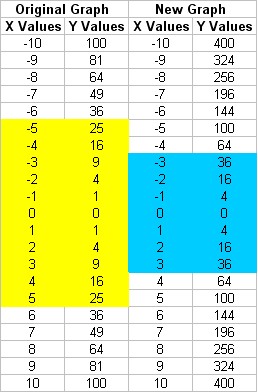
1) Generate a Table of Values
for y = (2x)2
The values shown in yellow are used for the original graph. The values
shown in blue are used for the new graph.
2) Plot the Graph of the
Original Function and the New Function
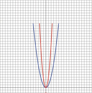
3) Compare the Graphs
The original graph is shown in blue, and the new graph is shown in
green. How does it compare?
The red parabola has the fewer data points than the blue one. The
shape looks quite different from the original graph; it has been
compressed and looks more narrow. It still has the same general shape,
though and it hasn't moved left or right.
|
y = f(x/3)
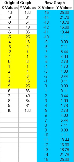
1) Generate a Table of Values for y = (x/3)2
The values shown in yellow are used for the original graph. The values
shown in blue are used for the new graph (rounded to two places).
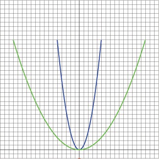
2) Plot the Graph of the Original Function and the New Function
3) Compare the Graphs
The original graph is shown in blue, and the new graph is shown in red.
How does it compare?
It appears as though the new graph is exapnded outwards. It uses more
data points, but has the same overall look.
|
The overall
effect appears to be that multiplying a constant term to the x value of
a function changes its shape. If the constant is
greater than 1, the graph becomes compressed inwards; if the constant is
less than 1, the graph expands in the x-direction. Result: y = f(cx) is similar to y = f(x)
but is either shifted or compressed in the x-direction.
Why does this happen?
When we evaluate the
new function, f(cx), we are changing what the function acts on. We are
changing the actual arguments (inputs) of the function.
Here are some
questions to ask:
1) If I know the
value of f(0) for the original graph, where does it appear in the new
graph for f(cx)? What new x value do
I need?
That same value of
f(0) in the original graph should appear at x = 0/c = 0. When we substitute x =
0/c into the new function we should get f (cx) = f (c × [0/c] ) =
f (0).
2) If I know the
value of f(3) for the original graph, where does it appear in the new
graph for f(cx)? What new x value do I
need?
The same value of
f(3) in the original graph should appear at x = 3/c. When we substitute x
= 3/c into the new function we should get f (cx) = f (c × [3/c] ) = f (3).
3) If I know the
value of f(-1) for the original graph, where does it appear in the new
graph for f(cx)? What new x value do I
need?
The same value of
f(-1) in the original graph should appear at x = -1/c. When we substitute x
= -1/c into the new function we should get f (cx) = f ( [c × -1/c] = f (-1).
We should see the same values of f(x) but
moved around to different x values
Notice that in each
of the answers, we divided by the value of c.
If c is greater than
1, multiplying by the
value of c gives us a larger number than our original x value. We can apply a kind of correction
factor by choosing a smaller
number than before to get the same result. The net result is that the
graph becomes compressed; we have to use smaller values of x to get the
same effect. If c is less than 1, multiplying by the value of c gives us
a smaller number than our original x value. We need to use a
larger input to compensate for this.This is why the graph
expands outwards; it needs bigger values of x to get the same results.
Here is a link to a summary page for these
various transformations.
On To the
Composite Examples
Back to
X-Coordinate Translations
Back to
the Introduction