X Co-ordinate
Changes: Translations
At this point, we know how to manipulate a function's y values through
the use of constant. These changed its y values or its vertical
appearance. Now will change the graph's horizontal shape and position.
These are given the general form of y = f(x+c), where f(x) is the
original function, and c is a constant value.
Let's take a look at two sample functions to see how it works.
|
y = f (x - 5)
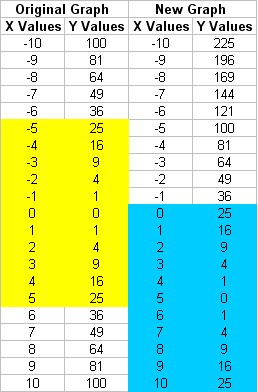
1) Generate a Table of Values
for y = (x - 5)2
The values shown in yellow are used for the original graph. The values
shown in blue are used for the new graph.
2) Plot the Graph of the
Original Function and the New Function
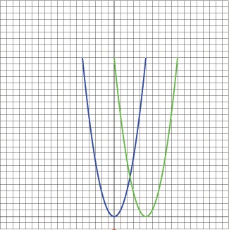
3) Compare the Graphs
The original graph is shown in blue, and the new graph is shown in
green. How does it compare?
The green parabola has the same amount of data points as the blue one.
However, we are using much higher x values than before to get the same y
values. Its shape looks exactly the same, but it looks like its been
moved to the right.
|
y = f(x - 9)
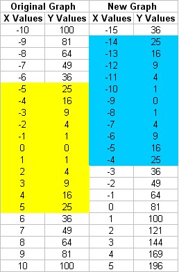
1) Generate a Table of Values for y = (x + 9)2
The values shown in yellow are used for the original graph. The values
shown in blue are used for the new graph.
2) Plot the Graph of the Original Function and the New Function
3) Compare the Graphs
The original graph is shown in blue, and the new graph is shown in red.
How does it compare?
Notice that the x-values in the table of values has shifted. The values
we are using are a lot less than in the original function. It appears as
though the new graph is shited to the left.The red function looks
exactly like the original blue graph.
|
The overall
effect appears to be that adding a constant term to the x value of a
function changes its position. If the constant is
positive, the graph moves to the left; if the constant is negative, the
graph moves to the right. Result: y =
f(x+c) is similar to y = f(x) but is moved left or right depending on
the value of c.
Why does this happen?
When we evaluate the
new function, f(x+c), we are changing what the function acts on. We are
changing the actual arguments (inputs) of the function.
Here are some
questions to ask:
1) If I know the
value of f(0) for the original graph, where does it appear in the new
graph for f(x+c)? What new x value do
I need?
That same value of
f(0) in the original graph should appear at x = - c. When we substitute x = - c
into the new function we should get f (x+c) = f ( [-c] + c) = f (0).
2) If I know the
value of f(3) for the original graph, where does it appear in the new
graph for f(x+c)? What new x value do I
need?
The same value of
f(3) in the original graph should appear at x = 3 - c. When we substitute x
= 3 - c into the new function we should get f (x+c) = f ( [3 - c] + c) =
f (3).
2) If I know the
value of f(-1) for the original graph, where does it appear in the new
graph for f(x+c)? What new x value do I
need?
The same value of
f(-1) in the original graph should appear at x = -1 - c. When we substitute x
= -1 - c into the new function we should get f (x+c) = f ( [-1 - c] + c)
= f (-1).
We should see the same values of f(x) but
moved around to different x values
Notice that in each
of the answers, the value -c appeared. If c is positive, we
need to move each point on the graph c units to the left (towards -c). This provides a kind
of correction factor. Since adding a positive number will increase the
value of the argument, we can move it towards a lower value to negate
its effects. If c is negative, move the graph towards -(-c) or +c to get the same y
values. Since adding a
negative number decreases the value of the argument, we can move it
towards a greater value to counter its effects.This causes a shift
to the right (in the positive x direction). Adding a constant
factor c to the argument of a function x causes this shift.
On To
X-Coordinate Scaling
Back to
Y-Coordinate Scaling
Back to
the Introduction