Without any predators, the prey would undergo exponential growth:
![]() , where
, where ![]() is a positive constant.
But predation reduces the growth rate or even makes it negative.
The simplest assumption is that the effect of predation is proportional
to both
is a positive constant.
But predation reduces the growth rate or even makes it negative.
The simplest assumption is that the effect of predation is proportional
to both ![]() and
and ![]() . Thus
. Thus
![]() .
As for the predator, without any prey it would starve, and
we assume this would happen exponentially:
.
As for the predator, without any prey it would starve, and
we assume this would happen exponentially: ![]() . But
with prey they can grow. Again the simplest assumption is that the
effect on
. But
with prey they can grow. Again the simplest assumption is that the
effect on ![]() is proportional to both
is proportional to both ![]() and
and ![]() :
:
![]() .
Thus we have the Lotka-Volterra equations, where
.
Thus we have the Lotka-Volterra equations, where ![]() ,
, ![]() ,
, ![]() and
and
![]() are positive constants:
are positive constants:
For an equilibrium point of the equations, we need ![]() or
or ![]() ,
and
,
and ![]() or
or ![]() . There are two equilibrium points:
. There are two equilibrium points: ![]() and
and
![]() . The Jacobian matrix is
. The Jacobian matrix is
 .
.
At ![]() the Jacobian matrix is
the Jacobian matrix is
 , with
eigenvalues
 ![]() and
and ![]() , one positive and one negative. Thus the origin
is a saddle point. The eigenvectors are
, one positive and one negative. Thus the origin
is a saddle point. The eigenvectors are
![]() for
for ![]() and
and
![]() for
for ![]() . Thus there will be
two trajectories entering the equilibrium point vertically (one up and one down)
and two leaving horizontally to the right and left.
. Thus there will be
two trajectories entering the equilibrium point vertically (one up and one down)
and two leaving horizontally to the right and left.
At
![]() the Jacobian matrix is
the Jacobian matrix is
 . The characteristic polynomial is
![]() . Thus the eigenvalues are pure imaginary:
. Thus the eigenvalues are pure imaginary:
![]() . In the linearization, this equilibrium point is
a centre. Unfortunately, this does not tell us whether the equilibrium
point in the nonlinear system is a centre or a stable or unstable spiral.
. In the linearization, this equilibrium point is
a centre. Unfortunately, this does not tell us whether the equilibrium
point in the nonlinear system is a centre or a stable or unstable spiral.
One way to resolve the question is to find an implicit equation that
![]() and
and ![]() satisfy. We find an equation in
satisfy. We find an equation in ![]() and
and ![]() by dividing
the second equation of our system by the first (pretending that
by dividing
the second equation of our system by the first (pretending that ![]() is a function of
is a function of ![]() ):
):


The isoclines for ![]() are
are ![]() and
and ![]() . Since
. Since ![]() is
a vertical line, there are
trajectories on it
(the two trajectories that enter the equilibrium point
is
a vertical line, there are
trajectories on it
(the two trajectories that enter the equilibrium point ![]() ).
The isoclines for
).
The isoclines for ![]() are
are ![]() and
and
![]() , so again there are trajectories on the
, so again there are trajectories on the ![]() axis
(the two that leave the
axis
(the two that leave the ![]() ).
).
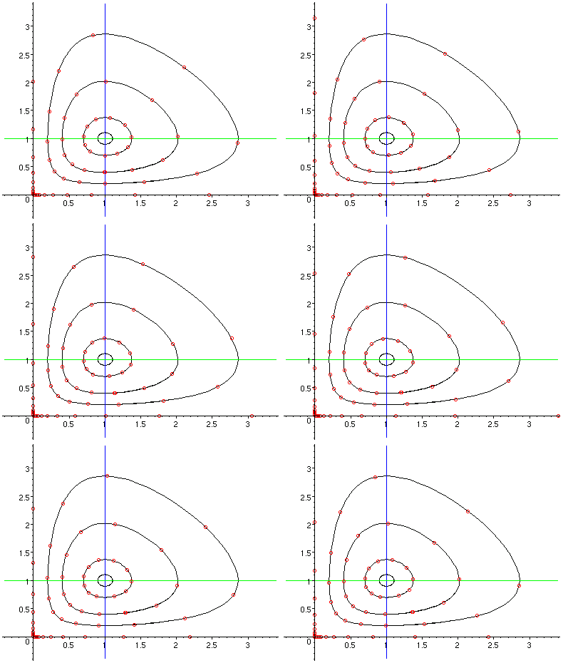
Here is the phase portrait of the system in the first quadrant, in the case
![]() :
:

Every trajectory in the first quadrant is a closed curve. Thus the
predator and prey populations oscillate go in cycles. Starting with a low
population of both predator and prey (in the region
![]() ,
,
![]() ), at first the prey increase while the predators decrease
(but not all the way to 0, because trajectories don't meet)
until
), at first the prey increase while the predators decrease
(but not all the way to 0, because trajectories don't meet)
until ![]() . As we cross into the region
. As we cross into the region ![]() ,
,
![]() the predators start to increase, while the prey
still increase until
the predators start to increase, while the prey
still increase until ![]() . Then we cross into
. Then we cross into ![]() ,
,
![]() , and the prey decrease while the predators increase until
, and the prey decrease while the predators increase until ![]() . Next, in the region
. Next, in the region
![]() ,
, ![]() , the predators
and prey both decrease until
, the predators
and prey both decrease until ![]() . Finally, in the region
. Finally, in the region
![]() ,
,
![]() , the prey increase while predators decrease,
and we come back to the start of the cycle.
, the prey increase while predators decrease,
and we come back to the start of the cycle.
It is not clear whether the cycles predicted by the Lotka-Volterra equation are observed in nature. There are species, such as lynxes and snowshoe hares in the Canadian arctic, that go through population cycles, but the fit between the data and the equations is not very good, and there may be complicating factors such as disease.
The closed curves of the Lotka-Volterra equations are a very ``delicate''
phenomenon, a consequence of the fact that the equation for ![]() happened to be separable.
Almost any modification to the equation would destroy this property.
We'll consider two modifications:
harvesting and self-limiting of the prey.
happened to be separable.
Almost any modification to the equation would destroy this property.
We'll consider two modifications:
harvesting and self-limiting of the prey.
Harvesting
First consider harvesting. We harvest prey at a small but constant rate
![]() .
Thus the equations become
.
Thus the equations become
Where are the equilibrium points?
For ![]() we still have
we still have ![]() or
or ![]() .
If
.
If ![]() , then
, then
![]() when
when
![]() . Thus the
equilibrium
point that was at
. Thus the
equilibrium
point that was at ![]() has shifted right to
has shifted right to
![]() . This is easy
to understand:
. This is easy
to understand:
![]() is just the population of prey for which, in the
absence of predators, the natural increase will just balance our harvesting
rate
is just the population of prey for which, in the
absence of predators, the natural increase will just balance our harvesting
rate ![]() . On the other hand, with
. On the other hand, with ![]() ,
,
![]() when
when
![]() . Thus the second equilibrium point has shifted
down to
. Thus the second equilibrium point has shifted
down to
 . We assume
 ![]() is small enough that
is small enough that ![]() .
.
The Jacobian matrix ![]() is still unchanged (because we have just added
a constant to
is still unchanged (because we have just added
a constant to ![]() ), but the equilibrium points have shifted.
For the first equilibrium point,
), but the equilibrium points have shifted.
For the first equilibrium point,
 .
The eigenvalues are
 ![]() , which is positive, and
, which is positive, and
![]() , which is negative
(again, assuming
, which is negative
(again, assuming ![]() is small).
So this equilibrium point is still a saddle. An eigenvector for the positive
eigenvalue is still
is small).
So this equilibrium point is still a saddle. An eigenvector for the positive
eigenvalue is still
![]() , and in fact
the trajectories leaving
this saddle point are still on the
, and in fact
the trajectories leaving
this saddle point are still on the ![]() axis (it is still true that if
axis (it is still true that if ![]() then
then ![]() ). An eigenvector for the negative eigenvalue is
). An eigenvector for the negative eigenvalue is
 ,
which (when
 ![]() is small) points up and slightly to the right.
is small) points up and slightly to the right.
At the equilibrium point
![]() , the Jacobian matrix is
, the Jacobian matrix is
 .
The characteristic polynomial is
![]() .
We have
.
We have ![]() and (when
and (when ![]() is small)
is small)
![]() , so this equilibrium point is an unstable spiral.
, so this equilibrium point is an unstable spiral.
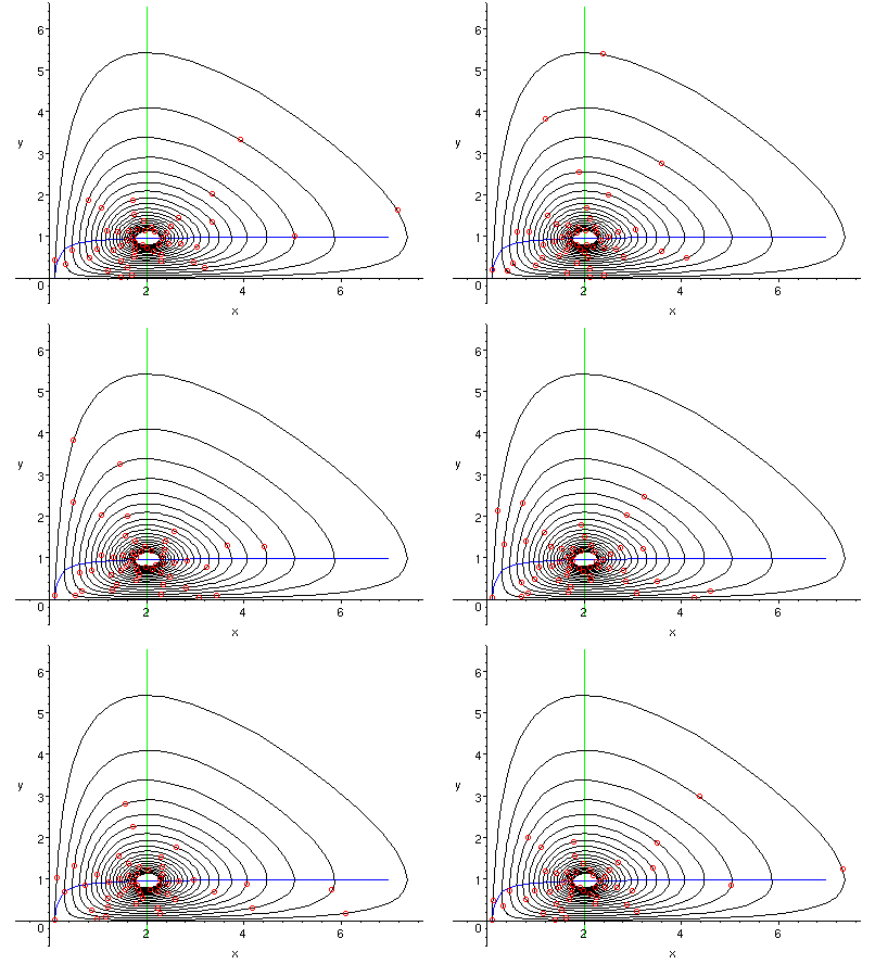
Here is the phase portrait, showing the trajectory that enters the saddle point.
Note that the isocline for
![]() is the curve
is the curve
![]() (shown in blue),
which has positive slope and goes through the two equilibrium points.
The isoclines for
(shown in blue),
which has positive slope and goes through the two equilibrium points.
The isoclines for ![]() are still the same as before.
Following backwards the trajectory that enters the saddle point from the
first quadrant, we see it spirals out of the equilibrium point
are still the same as before.
Following backwards the trajectory that enters the saddle point from the
first quadrant, we see it spirals out of the equilibrium point
![]() . The picture below is for
. The picture below is for
![]() ,
,
![]() ,
,
![]() . About 20 turns of the spiral are shown. Note that the
. About 20 turns of the spiral are shown. Note that the
![]() axis is not an isocline or a trajectory: trajectories can and do cross it.
Of course the equation does not make sense for
axis is not an isocline or a trajectory: trajectories can and do cross it.
Of course the equation does not make sense for ![]() , so what this means
is that the prey becomes extinct (and we then are forced to stop harvesting!).
In fact, for any initial condition in the first quadrant
that is not exactly on the trajectory that
enters the saddle point or at the equilibrium point
, so what this means
is that the prey becomes extinct (and we then are forced to stop harvesting!).
In fact, for any initial condition in the first quadrant
that is not exactly on the trajectory that
enters the saddle point or at the equilibrium point
![]() , the
solution will eventually hit
, the
solution will eventually hit ![]() , perhaps after spiraling a number of
times.
, perhaps after spiraling a number of
times.

A Self-limiting Term
At this point the future of our predator-prey system looks bad: even a
very small amount of harvesting causes the eventual extinction of the
prey (followed, of course, by the demise of the predator).
However, there
are other factors that can stabilize the populations. One such factor
is a self-limiting term for the prey, so that without predators or harvesting
it would undergo logistic rather than exponential growth. Thus we now take
Again we begin the analysis by finding the equilibrium points.
Again, either ![]() or
or ![]() to make
to make ![]() . If
. If
![]() , then
, then
![]() , which is a quadratic
in
, which is a quadratic
in ![]() . If
. If ![]() and
and ![]() are small,
are small,
![]() so there are two real roots, and both are positive (their product is
so there are two real roots, and both are positive (their product is
![]() , and their sum is
, and their sum is ![]() ). Thus we have two equilibrium points
on the positive
). Thus we have two equilibrium points
on the positive ![]() axis,
axis,
![]() and
and ![]() , where
, where

 .
.
At ![]() the Jacobian matrix is
the Jacobian matrix is
 . Since it is upper triangular, its
eigenvalues
are the diagonal entries
![]() and
and
![]() . The first
is positive, and (since
. The first
is positive, and (since ![]() is small when
is small when ![]() and
and ![]() are small)
the second is negative. So
are small)
the second is negative. So ![]() is a saddle point.
is a saddle point.
At ![]() the Jacobian matrix is
the Jacobian matrix is
 . Again the eigenvalues are on the diagonal,
and this time the first is negative but (since
 ![]() is large when
is large when ![]() is
small) the second is positive. So
is
small) the second is positive. So ![]() is also a saddle point.
is also a saddle point.
For both of these saddle points, an eigenvector for the first eigenvalue
is
![]() , and again the corresponding trajectories
are on the
, and again the corresponding trajectories
are on the ![]() axis, leaving
axis, leaving ![]() and entering
and entering ![]() .
.
At
![]() , the Jacobian matrix
is
, the Jacobian matrix
is
 . The characteristic polynomial is

Consider the case
![]() ,
, ![]() ,
,
![]() ,
, ![]() .
This has
.
This has
![]() , so
, so
![]() should be
a stable spiral. In fact, the Jacobian there is
should be
a stable spiral. In fact, the Jacobian there is
 , and its eigenvalues are
![]() . The equilibrium points are
. The equilibrium points are ![]() ,
,
![]() and
and ![]() . As we have seen,
the trajectories entering and leaving the saddle points are often
very important. In this case, it's particularly important to
see the relationship between the trajectories in the first quadrant
entering the first
saddle point
. As we have seen,
the trajectories entering and leaving the saddle points are often
very important. In this case, it's particularly important to
see the relationship between the trajectories in the first quadrant
entering the first
saddle point ![]() and leaving the second saddle point
and leaving the second saddle point
![]() . Both must hit the isocline
. Both must hit the isocline ![]() at some
point above the equilibrium point
at some
point above the equilibrium point ![]() . With the
help of a computer (calculating solutions numerically) we can
determine that the trajectory entering the first saddle point is
above the trajectory leaving the second saddle point.
In fact, it appears that the trajectory leaving the second saddle
point spirals in toward
. With the
help of a computer (calculating solutions numerically) we can
determine that the trajectory entering the first saddle point is
above the trajectory leaving the second saddle point.
In fact, it appears that the trajectory leaving the second saddle
point spirals in toward ![]() , while the trajectory entering
the first must continue along, with
, while the trajectory entering
the first must continue along, with ![]() and
and ![]() as
as ![]() . This trajectory is a separatrix: from any
initial point above it, the populations become extinct, while
below it they spiral in toward the stable equilibrium
. This trajectory is a separatrix: from any
initial point above it, the populations become extinct, while
below it they spiral in toward the stable equilibrium
![]() as
as ![]() . So the populations can survive
as long as they start out with enough prey and not too many
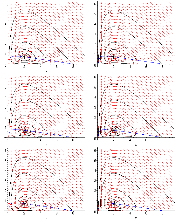
predators. Here is the phase portrait.
. So the populations can survive
as long as they start out with enough prey and not too many
predators. Here is the phase portrait.

If we increase the harvest rate ![]() to
to ![]() , keeping the
other parameter values the same, something new happens.
We still have three equilibrium points
, keeping the
other parameter values the same, something new happens.
We still have three equilibrium points
![]() ,
,
![]() and
and
![]() , and the first two are
saddles while the third is a stable spiral.
However, when the trajectories entering
, and the first two are
saddles while the third is a stable spiral.
However, when the trajectories entering ![]() and leaving
and leaving ![]() cross the isocline
cross the isocline ![]() , it turns out that the one entering
, it turns out that the one entering ![]() is lower. The result is that the trajectory leaving
is lower. The result is that the trajectory leaving ![]() continues
on and hits
continues
on and hits ![]() , while the one entering
, while the one entering ![]() goes into a spiral.
However, note that this one is spiraling outward, while near the stable
equilibrium point
goes into a spiral.
However, note that this one is spiraling outward, while near the stable
equilibrium point
![]() the trajectories must be spiraling
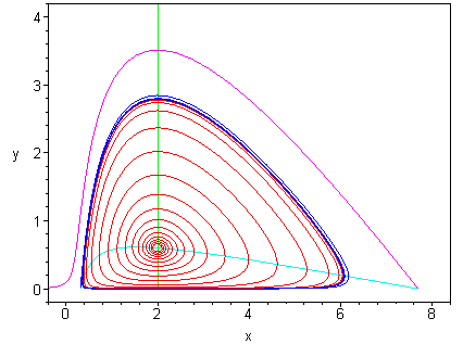
inward. How can these be reconciled? The answer is that somewhere
between them is a closed curve trajectory, called a limit cycle. Just outside
the limit cycle, trajectories spiral outwards, while just inside the limit cycle
they spiral inwards. Thus the limit cycle is a separatrix:
from any initial point inside the limit cycle, the
populations approach the stable equilibrium
the trajectories must be spiraling
inward. How can these be reconciled? The answer is that somewhere
between them is a closed curve trajectory, called a limit cycle. Just outside
the limit cycle, trajectories spiral outwards, while just inside the limit cycle
they spiral inwards. Thus the limit cycle is a separatrix:
from any initial point inside the limit cycle, the
populations approach the stable equilibrium
![]() as
as ![]() , while from any initial point outside the limit cycle (except those that
are exactly on the trajectory that goes in to
, while from any initial point outside the limit cycle (except those that
are exactly on the trajectory that goes in to ![]() ) they eventually become
extinct.
) they eventually become
extinct.
In the picture below, a trajectory spiraling inwards from the limit cycle
is shown in red, the trajectory entering the saddle point ![]() in blue, and the
trajectory leaving
in blue, and the
trajectory leaving ![]() in magenta. The limit cycle comes quite close to the saddle
point
in magenta. The limit cycle comes quite close to the saddle
point ![]() and the
and the ![]() axis.
axis.
