| Heun |
Euler |
Heun error | Euler error | ||
| 0.0 | 1.00000000 | 1.00000000 | 1.00000000 | 0.0 | 0.0 |
| 0.1 | 1.10511222 | 1.10000000 | 1.10526316 | 0.00015094 | 0.00526316 |
| 0.2 | 1.22185235 | 1.21022444 | 1.22222222 | 0.00036987 | 0.01199778 |
| 0.3 | 1.35225607 | 1.33223648 | 1.35294118 | 0.00068510 | 0.02070470 |
| 0.4 | 1.49886227 | 1.46792616 | 1.50000000 | 0.00113773 | 0.03207384 |
| 0.5 | 1.66487828 | 1.61959959 | 1.66666667 | 0.00178838 | 0.04706708 |
| 0.6 | 1.85441478 | 1.79009854 | 1.85714286 | 0.00272808 | 0.06704432 |
| 0.7 | 2.07282683 | 1.98296335 | 2.07692308 | 0.00409625 | 0.09395973 |
| 0.8 | 2.32722149 | 2.20265794 | 2.33333333 | 0.00611184 | 0.13067539 |
| 0.9 | 2.62723508 | 2.45488648 | 2.63636364 | 0.00912856 | 0.18147716 |
| 1.0 | 2.98626232 | 2.74704729 | 3.00000000 | 0.01373768 | 0.25295271 |
Clearly, in this example the Improved Euler method is much more accurate
than the Euler method: about 18 times more accurate at ![]() . Now if
the order of the method is better, Improved Euler's relative
advantage should be
even greater at a smaller step size. Here is the table for
. Now if
the order of the method is better, Improved Euler's relative
advantage should be
even greater at a smaller step size. Here is the table for ![]() .
.
| Heun |
Euler |
Heun error | Euler error | ||
| 0.0 | 1.00000000 | 1.00000000 | 1.00000000 | 0.0 | 0.0 |
| 0.1 | 1.10522508 | 1.10252967 | 1.10526316 | 0.00003808 | 0.00273349 |
| 0.2 | 1.22212855 | 1.21596496 | 1.22222222 | 0.00009367 | 0.00625726 |
| 0.3 | 1.35276701 | 1.34209198 | 1.35294118 | 0.00017417 | 0.01084920 |
| 0.4 | 1.49970962 | 1.48310373 | 1.50000000 | 0.00029038 | 0.01689627 |
| 0.5 | 1.66620837 | 1.64172213 | 1.66666667 | 0.00045830 | 0.02494454 |
| 0.6 | 1.85644079 | 1.82136643 | 1.85714286 | 0.00070207 | 0.03577643 |
| 0.7 | 2.07586420 | 2.02638978 | 2.07692308 | 0.00105887 | 0.05053330 |
| 0.8 | 2.33174590 | 2.26241822 | 2.33333333 | 0.00158743 | 0.07091511 |
| 0.9 | 2.63398036 | 2.53684738 | 2.63636364 | 0.00238328 | 0.09951625 |
| 1.0 | 2.99639263 | 2.85958887 | 3.00000000 | 0.00360737 | 0.14041113 |
As we saw before, in the Euler method the errors for ![]() are about
are about
![]() the errors at the same points for
the errors at the same points for ![]() . In the Improved Euler
method, the
. In the Improved Euler
method, the ![]() becomes
becomes ![]() (the actual ratio is from
(the actual ratio is from ![]() to
to ![]() ).
This supports the idea that Improved Euler's global error is
).
This supports the idea that Improved Euler's global error is ![]() .
.
For more support to this idea, we look at Improved Euler's error at ![]() as a function of step size
as a function of step size ![]() , using 14 different values for
, using 14 different values for ![]() :
:
![]() ,
, ![]() ,
, ![]() ,
, ![]() ,
,
![]() ,
, ![]() ,
, ![]() ,
, ![]() ,
, ![]() ,
, ![]() ,
, ![]() ,
, ![]() ,
,
![]() ,
, ![]() . We plot the error divided by
. We plot the error divided by ![]() : if the error is
approximately proportional to
: if the error is
approximately proportional to ![]() , this should be approximately constant.
, this should be approximately constant.
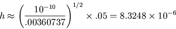
Now suppose we wanted the error at ![]() to be less than
to be less than ![]() .
For the Euler method, as we saw, we'd need more than 28 billion steps.
For Improved Euler, on the other hand, with error approximately proportional
to
.
For the Euler method, as we saw, we'd need more than 28 billion steps.
For Improved Euler, on the other hand, with error approximately proportional
to ![]() , we would need
, we would need
If the global error is ![]() , presumably the local error is
, presumably the local error is
![]() . Let's see this in the case of the differential equation
. Let's see this in the case of the differential equation
![]() . The Improved Euler calculation goes like this:
. The Improved Euler calculation goes like this: