First Order DE's and Direction Fields

A good way to think of the differential equation

$$\frac{dy}{dx} = f(x,y)$$

is that it tells you that at every point (x,y(x)) on a solution curve, the slope of the curve is f(x,y(x)).

Imagine that at every point of the x,y plane there is a little ``road sign'' that says, ``If you are here, go that way'' (indicating the direction corresponding to slope f(x,y)). The solution curve wanders over the x,y plane, following the road signs at each point it goes through. So if f(2,3) happens to be 4, and a solution curve passes through the point (2,3), it must have slope 4 at that point.

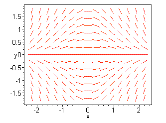
How could we sketch this situation? We might indicate the direction at a point by a short line segment through the point with the proper slope. We can't draw this for every point of the plane, but we could take a representative selection of points (perhaps in a rectangular grid on part of the plane), and draw those. Here is a typical example, for the differential equation

$$\frac{dy}{dx} = - x y$$

as plotted by Maple.

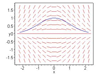
Imagine starting at a point in the plane, say (0,1), and moving to the right following the direction field, as the solution curve must do. At (0,1) itself the slope is , but as we pass into the first quadrant the slope becomes negative, and we curve downward. However, we never reach the x axis, as the slope becomes gentler as we approach y=0. The x axis will be a horizontal asymptote.

Similarly, we can start at (0,1) and move to the left, following the direction field backwards. As we pass into the second quadrant the slope becomes positive, we curve downwards, and then approach the negative x axis as a horizontal asymptote. Putting the forward and backward curves together, we have a sketch of the solution curve.

The basic principles of sketching solution curves from direction fields are as follows:

• Through every point (x,y) where f(x,y) is continuously differentiable there is a unique solution curve, whose slope follows the ``road signs''.
• Solution curves can't stop, except by either going off to infinity or encountering a point where f(x,y) is not continuous.
• Solution curves can't meet or cross, except at a point where f(x,y) is not continuously differentiable.

These principles follow from the Existence and Uniqueness Theorem for differential equations (Theorem 2.11.1 in the text).

In our example, the x axis itself is a solution curve, i.e. y=0 is a solution. Therefore principle (3) guarantees that the solution curve through (0,1) never hits the x axis.

Instead of sketching the direction field using line segments, we often draw isoclines, which are the curves f(x,y) =constant. The most important value for the constant is usually 0, which tells where the solution curves have horizontal tangents. The isoclines divide the plane into regions, in each of which the slopes are between certain bounds. The next plot shows the isoclines in our example for slopes 0 (in green), 1 (red) and -1 (blue), together with two solution curves in black. Note that in general the isoclines are not solution curves.

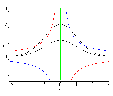
Let's follow the top solution curve to the right from (0,2). Since this point is on the isocline for slope 0, there is a horizontal tangent there. As we pass into the region between the green and blue isoclines, the slope is between 0 and -1. The curve bends downward. Since the slope is greater than -1 in this region, we must hit the blue isocline (to avoid it, we would need to go below the straight line from (0,2) to (1,1), but that line has slope -1). After crossing the blue isocline, we are in a region where the slope is less than -1. Clearly we must then hit the blue isocline again, at some point to the right of (1,1). We then pass again into the region where the slope is between 0 and -1, and must stay there, trapped between the blue isocline and the x axis.

On the other hand, the solution curve that passes through (0,1) never hits the blue isocline. It also can't meet the solution curve that goes through (0,2) (although they get so close to the x axis as $x \to \infty$ that they and the axis may appear to meet).