Constant-Coefficient Equations
Second-order linear equations with constant coefficients are very important,
especially
for applications in mechanical and electrical engineering (as we will see).
The general second-order constant-coefficient linear equation is
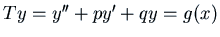 , where
  and
and  are constants. We will
be especially interested in the cases where either
are constants. We will
be especially interested in the cases where either  (the
homogeneous case) or
(the
homogeneous case) or
 for some constant
  .
The main idea in solving these equations is:
make an educated guess at the form of the solution, and see what has to
happen to make a function of this form satisfy the equation. In the
homogeneous case,
it turns out that the form to use is
.
The main idea in solving these equations is:
make an educated guess at the form of the solution, and see what has to
happen to make a function of this form satisfy the equation. In the
homogeneous case,
it turns out that the form to use is
 , where
  is a constant. If we plug this in to the
differential equation, we get
is a constant. If we plug this in to the
differential equation, we get
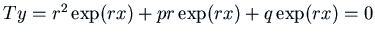 , and factoring out
the
, and factoring out
the  (which is not
  ) we are left with
This is called the characteristic equation of the operator  (or of the
differential equation). If is a root of the characteristic equation,
is a solution of the differential equation.
Recall that we are looking for a fundamental set consisting of two
linearly independent solutions. Now a quadratic equation may have two
real roots, and this would give us our two solutions (it is not hard to see
that they are linearly independent).
Example: Consider the equation
(or of the
differential equation). If is a root of the characteristic equation,
is a solution of the differential equation.
Recall that we are looking for a fundamental set consisting of two
linearly independent solutions. Now a quadratic equation may have two
real roots, and this would give us our two solutions (it is not hard to see
that they are linearly independent).
Example: Consider the equation
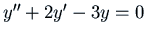 . The
characteristic equation
. The
characteristic equation
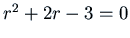 has two roots
  and
and
 . Therefore
  and
and  form the fundamental
set of solutions. The general solution is
form the fundamental
set of solutions. The general solution is
Now, a quadratic equation may also have only one real root, or no real
roots. We will have to deal with these possibilities as well.
At this point it is useful to introduce the differentiation
operator  defined by
  . We can then write the operator
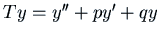 of our differential equation as
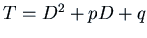 , a polynomial in . We can manipulate polynomials
in just as we would manipulate ordinary polynomials. For example,
we might factor
, a polynomial in . We can manipulate polynomials
in just as we would manipulate ordinary polynomials. For example,
we might factor
 .
What does
.
What does  mean? These are operators, so they are defined
by what they do to functions. The ``multiplication'' of operators
is really composition: you first let the operator on the right
act on the function, and then the operator on the left acts on the
result. Thus for
mean? These are operators, so they are defined
by what they do to functions. The ``multiplication'' of operators
is really composition: you first let the operator on the right
act on the function, and then the operator on the left acts on the
result. Thus for  you first take
 , then
 .
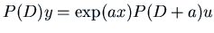
The characteristic polynomial is related to the way the operator
acts on exponential functions:
.
The characteristic polynomial is related to the way the operator
acts on exponential functions:
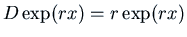 .
So, for example,
.
So, for example,
 . Or in general, for any polynomial
  ,
,
This has the following consequences:
- If
 then is a solution of the
homogeneous equation
then is a solution of the
homogeneous equation  .
.
- If
 then
one solution of the non-homogeneous equation
then
one solution of the non-homogeneous equation
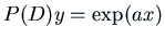 is
is
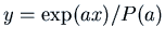 .
.
Now how can we deal with the homogeneous equation when  has only one real root, or with the non-homogeneous equation
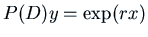 where ? The key is the
Exponential Shift Theorem: For any polynomial , constant
where ? The key is the
Exponential Shift Theorem: For any polynomial , constant  and function
  ,
,
Proof: Note that
 .
Repeated application of this gives us the result for any power of , e.g.
.
Repeated application of this gives us the result for any power of , e.g.
Adding constants times powers of gives us all polynomials.
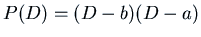
Now let's apply this to where the polynomial  has only one root.
This means
has only one root.
This means
 where is the root. We look for a solution
of the form
where is the root. We look for a solution
of the form
 for some function . The Exponential Shift
Theorem says
for some function . The Exponential Shift
Theorem says
 , so we want
  .
Two linearly independent solutions of this are
.
Two linearly independent solutions of this are  and
and  .
Thus a fundamental set of solutions of
.
Thus a fundamental set of solutions of  is
is  and
and  .
.
Similarly, we can try
where  . Again we try
, and get
. Again we try
, and get
 , so we want
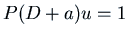 .
.
- If
 with
with  ,
,
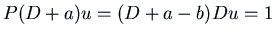 .
Writing
.
Writing  we want
  . Clearly one solution of this
is the constant
. Clearly one solution of this
is the constant  . Then from
  we get a solution
 , i.e.
 .
.
- If
 ,
,
 . Clearly one solution
is
. Clearly one solution
is  , i.e.
 .
.
Example: Solve the initial value problem
We have
 , with one root
  .
Since the right side of the equation involves , we use the
Exponential Shift Theorem with
.
Since the right side of the equation involves , we use the
Exponential Shift Theorem with
 . We have
 , so one solution is
  . This gives
us one solution of our differential equation:
. This gives
us one solution of our differential equation:
 . The fundamental set of
solutions of the homogeneous equation
. The fundamental set of
solutions of the homogeneous equation  is
is
 and
and  . Thus the general solution is
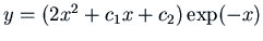 . From the initial conditions we
have
. From the initial conditions we
have
 and
and
 . Thus
  and
and
 , and the answer is
Robert Israel
2002-02-07