The Closest Point Method

The Closest Point Method is a new technique for computing on surfaces. For example, the Closest Point Method could be used to compute a numerical solution of a partial differential equation on the surface of a sphere, torus, Möbius strip, or human hand. The animation on the right shows the motion of an interface (shown as the transition from between black and white) on the surface of Laurent's Hand. The interface is moving normal to itself (so-called unit normal flow) and is an example of the level set method applied on a surface.

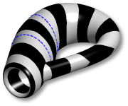
Torus

Unit normal flow on the surface of a torus (left). The interface (shown here as the black contour on the transition from blue to red) starts at the left and moves rightward by unit normal flow, separates into two interfaces in the middle, and finally rejoins into a single interface at the right.

See the animated torus (also in mpeg format)

Klein bottle

Redistancing (computing a signed distance function) on the surface of the Klein bottle (right). Each transition from dark-to-light or light-to-dark represents contours of equal distance from the closer of the two initial interfaces indicated with dashed blue lines.

See the animated Klein bottle (mpeg).

The Klein bottle is a codimension-two surface in 4D with no inside/outside; the Closest Point Method is extremely flexible with respect to surface geometry.

Forest Fires: level sets on surfaces

Simulated forest fire on a hill: mountain_slope3.mpg. The flame front is represented by the zero contour of a level set function. The model (which is not necessarily physically realistic) specifies that the flame front wants to spread outwards in the in-surface normal direction and also spreads faster in the uphill direction. The numerical computation is performed in Matlab using Ian Mitchell’s Toolbox of Level Set Methods.

This computation was motivated by work during the 2007 MITACS Industrial Math Summer School with Helen Alexander, Anna Belkine, Chris Poss, and Weining Wang.

Blurring with the heat equation

Solving the heat equation blurs the phone number written on Laurent's hand. The images on the right show the initial conditions and the progressively blurrier results after 1, 2 and 6 time steps. For this problem, implicit time stepping allows relatively large time steps compared to explicit methods.

Flexible computational domains

The tail of Annie Hui’s pig is connected to a sphere by a long filament (infinitesimally thin wire). A heat source is then applied under the sphere. The temperature over the entire surface of the domain is modelled according to the heat equation with a localized source term (using Newton’s law of heating and cooling) to account for the candle.

The temperature is initially zero, the candle has temperature 10, and this animation (mpeg) shows the change in heat until t=25. The figure on the right shows the temperature on the surface of the pig at this final time.

This surface is comprised of components of various codimension (the pig and sphere are codimension 1 whereas the filament is codimension 2). This poses no difficulty for the Closest Point Method and the computation proceeds exactly as it would for a simpler surface.

The “Bunnyator” or the “Brusselhare”

Solutions of the Brusselator reaction-diffusion system on the surface of Stanford Bunny can exhibit various pattern formation behavior. For different values of the parameters, the image on the right shows honeycomb, stripes and spots on the bunny surface. An animation (mpeg) shows the solution evolving in time.

Biharmonic problems

Solving in-surface biharmonic (fourth-order) problems is a one-line change in the code: we simply square the matrix used for the Laplace--Beltrami operator.

The image on the left shows the evolution of a fourth-order interface motion problem on a bumpy sphere. This example uses an innovative semi-implicit splitting by Peter Smereka.

Luke Tian's MSc thesis applied the Closest Point Method to the problem of image segmentation. Luke used the Chan-Vese segmentation algorithm—adapted to surfaces using the Closest Point Method—to detect objects in the textures of surfaces.

The figures on the left and right (both made by Luke) demonstrate the results: in each case a contour evolves, eventually separating the surface into two distinct regions. In the case of the pig, into red and blue.

The article Segmentation on surfaces with the Closest Point Method (Luke Tian, Colin Macdonald and Steve Ruuth) has been submitted for publication.

Eigenvalue problems

The Closest Point Method can be used to solve surface eigenvalue problems. The images on the left show some Laplace--Beltrami eigenmodes of a Mobius strip. These can be thought of as vibration patterns of a stylized Mobius-shaped drum.

The figure on the right shows the first nine eigenmodes of continental Africa. The computation is performed using an Africa-shaped piece of a sphere using the Closest Point Method. Dirichlet boundary conditions are applied along the coast line.

The results modes can be compared to the well-known problem of eigenmodes of a L-shaped domain. Interesting to note that they are fairly similar.

Tom März has looked at the underlying mathematics of the method and presented proofs of the principles needed for the Closest Point Method.

Steve Ruuth’s website has other Closest Point Method pictures and animations.