Mathematics 309- the elementary geometry of wave motion

Mathematics 309 - the elementary geometry of wave motion

Part I - Scaling and Shifting

Part II - Elementary Wave Functions (1D)

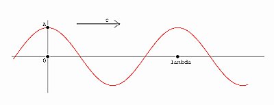
This is an example of simple periodic motion in one dimension (1D). The motion can be described using the parameters

, c, A,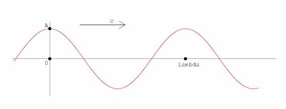

where

is the radial frequency (ie measured in radians per second,

(lambda on the graph) is the wavelength which is the distance from one peak to the next, c the velocity (or speed in 1D) of the wave and A the amplitude or height of the wave.

A relationship can be found between these parameters using the basic equation of motion: Speed = Distance/Time. For our case, the distance is , linear frequency is the inverse of the time it takes to travel that distance. Radial frequency is 2 times the linear frequency. So the relationship is: c = / 2. It shall be seen later that as Velocity = Displacement/Time this also works for 2- and 3D.

The wave equation

The picture above can be described with a mathematical equation. One can see the basic shape of the graph is a cosine wave. Using the methods of scaling and shifting described in part I the equation of a general wave function with unspecified parameters can be found.

The basic equation at the start is

y = cos(x). As time runs, the graph shifts right by ct at time t, so similar to the fourth set of pictures in part I, x-ct is substituted for x. The new equation is

y = cos(x-ct).
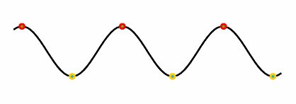
A normal cosine wave has a period of 2

, but an equation is needed for any wavelength

. Thus the third set of pictures shows the need to substitute 2

for x to get a horizontal scaling of

. Therefore the equation is more generally

y = cos(2(x-ct)/) = cos(2x/ - 2ct/) .
Next, variable amplitude A is needed instead of a unit amplitude. Similarly to the first set of diagrams in part I, the function is multiplied by a constant to get

y = Acos(2x/ - 2ct/) or, from above, y = Acos(2x/ - t).

Part III - Affine Functions and 2 and 3D

Now waves in more than one dimension will be studied; the following diagrams illustrate a plane wave in 2D from two views; top and side. A 3D wave will have a velocity and wavelength acting in 3 dimensions, an example could be of waves radiating out from a sphere rather than a plane source. The wavelength and velocity in 2 and 3D will be vectors instead of scalars, to show the magnitude and direction of these parameters. It is known that the fundamental equation c = / 2 still applies, but in vector form.

Affine functions can be used to describe the wave height as a function of space and time. Recall that affine functions are transformations that preserve colinearity and the ratio of distances so that an object's intersection properties remain unchanged. The general form is Ax + By + Cz + D.
A generalized formula for the height is y = Kcos(Ax + By + Cz + Dt), where K, A, B, C, D are constants to be determined. Obviously this is a case for 3D waves; 2D is just without the cz term. In this chapter 3D versions will usually be given; the 2D versions are similar, but again, without the z term.

At time t=0, y = Kcos(Ax + By + Cz). The argument of cos is called the phase, and varying the values of A, B, C gives different phases. This produces the parallel lines (or level lines) forming the crests of the waves shown in the first picture above.

If the general form of an affine equation above is taken, the constants can be identified: [A, B] (and similarly [B, C] and [A, C] in 3D) is the normal vector to the parallel lines. This is because
[A, B].[x, y] = Ax + By = 0 is the line y = Ax + By + Cz + D through the origin in two dimensions.
also has meaning in terms of A, B, C, D. Using Pythagoras, it can be worked out that
= D/ sqrt(A² + B² + C²). is always the wavelength vector perpendicular to the level lines.
For a wavelength of magnitude 2, the wavelength has vector 2[A, B, C] / (A² + B² + C²). So the wave height has a function y = Kcos(Ax + By + Cz) at t=0 with [A, B, C] related to .
For any time, the wave height is y = Kcos(Ax + By + Cz - t) where is the radian frequency.

Sources:

MATH 309 Wave Motion