
Figure 4.1
| The 2D wave equation |
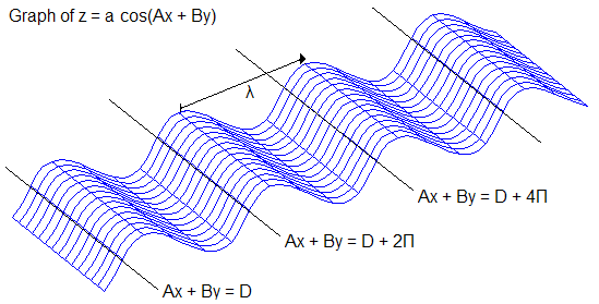
a cos(Ax + By),where a is the amplitude. It gives a graph like the following:
|
Figure 4.1 |
|
|
|
In 2 dimensions, the wavelength λ becomes a vector, as we see in Figure 4.1. It expresses the distance and direction from the crest of one wave to the crest of the next. Note that λ is perpendicular to the level lines of Ax + By.
| Calculation of λ |
We know from Part III that the signed distance from level line Ax + By = 0 to level line Ax + By = 2Π is
2Π / √(A2 + B2).This is the length of λ, since it is the distance between crests. To find λ itself, we simply normalize the vector [A, B] to get a unit vector
[A, B] / √(A2 + B2).This vector has length one and points in the direction of λ, so we simply scale it by the length of λ to get λ:
λ = 2Π [A, B] / (A2 + B2).
| Moving with time |
a cos(Ax + By - ωt).
| Extending to 3D |
a cos(Ax + By + Cz),
λ = 2Π [A, B, C] / (A2 + B2 + C2), and
a cos(Ax + By + Cz - ωt).