Waves in Higher Dimensions (2D and 3D)

Starting with the wave equation in one dimension, we can extend it into greater dimensions. Due to graphical limitations, it is difficult to draw multi-dimensional waves. As such, they are often schematically drawn as follows:


The motion of the wave is drawn in red. In a multi-dimensional environment, the wave will also have depth (that extends into the computer screen). Instead of drawing the entire wave, we just draw the blue lines above to denote the crests of the wave as they move through the 3D environment. As this point, we introduce the concept of affine transformations and affine functions. They will prove to be very useful in describing and generating the wave equation in higher dimensions.

Affine Transformations and Functions

Given a function Ax+By = C, how can we graph it? In general, we can plot out a set of values. However, this is very tedious, and is too specific to be of any general use. We can modify the formula into the form y = mx +b , where m equals the slope, and b is the y-intercept. When we try to solve for the function in y, we run into a distinct problem.

Ax+By = C
By = C - Ax
y = -(A/B)x + (C/B) = mx + b

For most choices of A,B, and C the function is well defined. However, if B equals zero, then this equation fails since you cannot divide through by zero. We would then have to augment the equation as follows:


Ax+By = C
Ax+(0)y = C
Ax = C
x = (C/A)

For any general equation, it is inconvienent to constantly need to consider two cases.  Another method is required, we can first change the given function of
Ax+By = C by re-writing as Ax+By - C = 0.  At this point, we'll consider the general case where C = 0.

When C = 0, the function reduces to Ax + By = 0. We can plot this function by first graphing the line (or vector) [A,B], and then drawing the line perpendicular to it that goes through the origin.
We can see that this general method works based on the first equation for the line that we obtained: y = -(A/B)x + (C/B). The vector [A,B] has slope B/A, and the slope of the curve is -(A/B).  The product of these slopes is -1, which is the condition for perpendicular lines.

This method has the additional advantage in that it corrects against the case where B = 0 because the vector [A,0] is simply the x axis, and the vector perpendicular to it is the y axis. If A and B equal zero, then the equation represents the origin, and is the degenerate case 
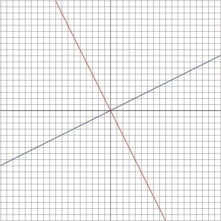
where the line becomes a single point. The following is a graphic where the blue line represents the vector [2,1], and the red line is graph of 2x + y = 0 (You can also see that the red line has slope of -2, and is indeed perpendicular to the blue line).


While we have considered the simple case of C = 0, we also need consider cases where C is non-zero. The first thing that we should notice is that the formula y = -(A/B)x + (C/B) guarantees that as long as we can draw vector [A,B], the line of any Ax+ By = C will be perpendicular to it. We need to see how the constant value C will augment the original line where C = 0. Here's a graph of the lines 2x + y +C = 0, where C = ±15, ±10, ±5, ±4, ±3, ±2, ±1 and 0. From left to right, the value of C increases, starting from -15 on the far left to 15 on the far right. Each of lines remains parallel (as predicted by the slope equation). It also appears as through the lines are spaced apart relative to the value of the constant value, C.


This allows to interpret the general relation where we can graph Ax+By=0, and then apply a correction factor for the constant.The value of the distance (through the perpendicular) between each pairing of lines is given by:

Distance = C2-C1  /[sqrt(A2+B2)] or when C1 equals 0, C2 /[sqrt(A2+B2)]

In this formula, if C is positive the graph will be above the graph of Ax+By=0 towards the right, and in the direction of [A,B]. If C is negative, then the graph is left of C = 0.

The Wave Equation in Higher Dimensions

We can use the result of the wave equation to solve the wave equation in higher dimensions.


As above the red curve represent a part of a three dimension wave that we can view. The blue represent the crests of waves are hidden behind the front one. There is a marker for the  wavelength λ, which represents one period of the wave. We can see that the crests of the wave are very similar to the parallel lines from the example that we used for the affineλ transformation constant determination. In fact, λ happens to be perpendicular to the waves, in a fashion similar to [A.B] in the previous case, and is regarded as a multiple of [A.B].

We can write down some relations:

λ = k [A,B]
 
where k is a constant, and [A,B] is perpendicular to the direction of motion (from the definition of λ)

We now take the length of λ as defined by the direction of motion to get:

║λ║ = k [sqrt (A2+B2) ]

If we calculate the signed distance of
λ based on its similar to C (for a given C) we get:

║λ║ = C  / [sqrt (A2+B2)]


Now we equate the two expressions for the length of λ:

║λ║ = C  / [sqrt (A2+B2)] = k [sqrt (A2+B2) ]

If we solve for k we get:


k = C / A2+B2
As a result, the equation for λ is given by:

λ = k [A,B] = C / A2+B2× [A,B]

At time = 0, the wave height equation for a 2D time independent curve is given by h(x,y) = A cos (ax + by). This is the same as in 1D case , but with an extra factor for the y-dimension. As in the 1D case, we can now apply the radian frequency correction factor to generate our final equation of:

h(x,y) = A cos (ax + by - ωt),
where a and b are constants, and ω is the radial frequency function (
2πc/λ).

This equation can be raised into any number of dimensions by adding more dimension terms with constants.