Waves in 1 Dimension

Using our knowledge of general function transformations, we can change simple functions into more complex ones. In this case, we are going to use a cosine curve as a model for wave behaviour in one dimension. Let's take a look at some of the key features of a standard cosine curve.


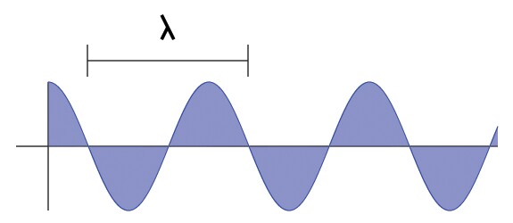
A cosine curve is a periodic function. Over a given amount of time, the function will repeat itself into identical copies, called periods. As you can see, the function resembles a wave. The standard cosine function is based on the unit circle. There are two ways to consider the behaviour of the periodic function.

Time Independent/Position Dependent
Assume that the above graphic has position in the y axis, and the x-axis represents the position of curve. Time is held constant in this equation; imagine that the graphic represents a snapshot of a moving wave at any point in time. Starting from
x = 0, the graph takes the value of the x-coordinate as the radius moves around in a counter-clockwise fashion until it returns to its initial starting place.

Time Dependent/Position Independent
Assume the above graphic has position in the y axis, and time in the x-axis (as time increases, the graph moves to the right). The position of interest is held constant in this case. A good example would a Ferris Wheel. Imagine that you are sitting in the same spot in the Ferris Wheel (as is usually the case); your position is now fixed in your seat. As time progresses, the chair begins to move up and down relative to the ground as Ferris Wheel rotates. The above graphic tracks your progress as you oscillate up and down. Your position remains the same, but your height is changing with respect to time.

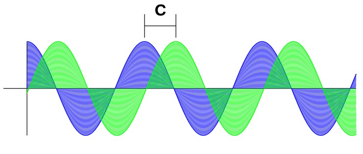
In any case, the curve that is traced out is the same. This co-dependence allows the wave equation to be properly expressed as y(x,t). However, we will begin our look with the analysis of the wave equation in 1D. Because it is easier to visualize, we will use the time independent equation. There are a few ways to change the visual appearance of a standard wave.


Current Formula: y = cos x

Amplitude


The easiest way to alter the appearance of a cosine curve is to modify its amplitude. By multiplying the entire function by a constant, A, the height of the function is scaled. When A is greater than 1, the maximum height increases; when A is less than 1, the maximum height decreases. In the above picture, the pink/salmon coloured curve (the tallest one) corresponds to A = 2. The purple cosine curve (medium sized) is when A = 1, and the grey-blue curve (smallest) occurs when A = 0.5. We can add this factor into our wave equation.

Current Formula: y = A cos x

Wavelength


That strange looking symbol above the curve is lambda ( λ ).
λ is used to represent the wavelength of a function. The wavelength of a function refers to the distance (length) that defines one period of the function. For the standard cosine curve, its value of lambda is 2π. Over the course of 2π radians, the function will repeat itself. In order to modify the wave equation, we can multiply the x argument 2π. This would cause the period of a cosine curve to go from being [0,2π] to [0,1]. This is since each value of [0,1] maps to a unique value in [0,2π] so the function remains the same general shape, but scaled inward.

Current Formula: y = A (cos [2πx] )

We can further modify this by dividing the value of the argument of function by dividing by any desired λ. This forces the range from [0,1] to [0,λ]. This means that each value of [0,λ] will now map to a value in the interval of [0,1]. This effectively generates the desired curve for any given wavelength λ.

Current Formula: y = A [cos (2πx/λ) ]

Time Shift


As with other translations, we may wish to translate the curve along the x-axis. This keeps the original shape of the curve, but translates it by c units to the left (if c is positive) or to the right (if c is negative). The value of c is known as the time shift because it changes the graph by varying the distance between the two curves over a varying amount of time. The value of the shift can be seen by finding the same point in the two graphs and measuring the distance between them. In the above graphic, the difference between the two crests can be used to find the value of c.

Current Formula: y = A  [cos 2π/λ (x-ct) ] OR y = A  [cos (2π/λx-2πc/λt)]

Radian Frequency

There is an interesting quantity that arises from this formula. The constant portion of the argument of the current formula (2πc/λ) has units in frequency (Time)-1 that when multiplied by  time yields a constant (which makes sense since we are taking the cosine of this quantity). A common measure of this unit is Hz or s-1 which is commonly used to express the number of occurrences per second. The value of this constant 2πc/λ is known as the radian frequency, and is typically denoted by the Greek symbol lowercase omega, ω. It turns out that the quantities c and λ have units that will cancel out and become 1/Time.

ω = 2πc/λ = [(constant) (distance/time)] / (distance) = (constant)/Time  ... which is proportional to Time-1


The radian frequency is a useful quantity because it allows one to more accurately describe the rate of rotation of an object. For example, when one quotes a velocity of an object, it does not give a notation of an object's rate of rotation. Take the given example below.


From the diagram, there are two arcs (red and blue) that sweep out an angle (θ) over a given amount of time. While both angles sweep out the same angle, an object travelling along the red path must have a higher velocity than an object on the blue path. The distance contained in the red arc is greater than that of the blue arc, so for a fixed amount of time, the red object must travel faster. Radian frequency allows one to describe how fast an object is rotating or how many periods it completes in a given amount of time.

Now that we have established the wave equation in one dimension, we extend it into higher dimensions.

On To Wave Equations In Higher Dimensions
Back to Composite Functions
Back to the Introduction