Effects with Cassini Ellipses
Liquid Effects
By: Arsham Skrenes
To take things to the next level, I thought it would be interesting to use Cassini ellipses to simulate fluids. One could also use this technique to simulate electron density maps. Before doing that, however, there are a few important things regarding implementing the Cassini ellipses. In order to use them in 2D/3D it would be best to use parametric equations:
Where  and b > 0
However, there are additional restrictions...
 . I found that it is better to explicitly set this otherwise rounding errors can result in errors (due to imaginary numbers).
 Finally, a mirror copy of the function must be created on the other side of the y-axis.
The result can be viewed by clicking on the following:
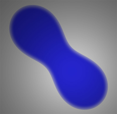
Of course for multiple-interacting elements, the proper way to do this is by creating metaballs and using a walking-cubes algorithm. However this is a very CPU and memory intensive endeavor. For simplicity, using Cassinis ellipses certainly does a good job.
This last demonstration is done completely in 3D. However, it isnt perfect but shows how one could use a combination of techniques to have a perfect solution for whatever application (whether it be electron density clouds or simply mud). In this demo, the Cassini ellipses do not take over until contact has been made between both objects.
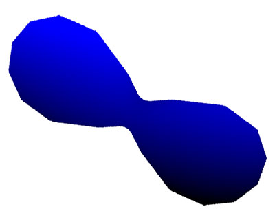
Incidentally, this demo was done quite rapidly; as a result, there are major limitations with it. However for the sake of demonstration, it shows that this can be done in 3D, even with postscript.